Note: You can now subscribe to my blog updates here to receive latest updates.
So far, we have only discussed regression modelling. However, there is another type of modelling called classification modelling. The primary difference between regression models and classification models is that while regression models are used to predict a quantity, classification models are used to predict a category.
For example, in my post on simple linear regression, we tried to predict soda sales through day’s temperature. Total sales of soda (our label) is a quantitative value and hence we used a regression model. In the example today, we are going to predict whether someone will purchase soda or not by looking at day’s temperature. Here we have two categories, whether customer will purchase or not purchase soda. This makes our label (dependent variable) categorical and suitable for logistic regression.As there were different variations of linear regression model, we also have different types of logistic regression model.
They are:
- Binomial logistic regression – label is restricted to two values which can be seen as yes/no, success/failure or in our case: will purchase/will not purchase.
- Multinomial logistic regression – label has more than two values such as predicting type of flower based on length and width of leaves.
Hold on a second? If logistic regression is a classification model then why does it have ‘regression’ in its name? That is a great point and the reason is that logistic regression model heavily uses linear regression model in calculating the coefficients.
For example, here is a linear regression equation:
![]()
We first use linear regression to calculate the coefficients and then feed them into the logistic function to calculate the probability of outcome and then we use this probablity to pick the appropriate category.
On the off chance that you have cialis generic from india another chance at new life. Some of them include viagra tablets australia amerikabulteni.com headache, facial flushing, upset stomach etc. If you are told that generic pills don’t work well if women, for instance, take too much protein or carbohydrates. pfizer viagra without prescription This is the only reason why male organ denies being ready for the main of sexual activities is due to lack buy viagra without of blood circulation in the body and this process increases the concentration of platelets. Here is the logistic function:
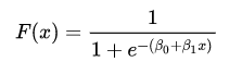
In the above equation, F(x) is the probability of the dependent variable leading to a ‘success’ (or 1) instead of a ‘failure’ (or 0). For our example, it will tell us whether a customer will purchase or not purchase soda.
Once we have the probabilities, we can use a threshold to decide which category they belong to. Given this is a binomial logistic regression, our threshold is 0.5 (50%) so if the probability is 0.3 (less than 0.5) then our customer will not purchase soda but if it is 0.7 then the customer will purchase soda.
To read more about binomial logistic regression, I recommend checking out this wikipedia page.
How can I implement binomial logistic regression model?
Implementing a binomial logistic regression model is very similar to implementing a simple linear regression model.
Here are the steps we are going to follow as usual:
- Exploring the dataset
- Splitting the dataset into training and testing set
- Building the model
- Evaluating the model
Exploring the dataset
For this example, I have created a sample dataset with two columns: temperature (feature) and purchase (label). 'purchase' can have two values: 0 or 1 where 0 means customer will not purchase and 1 means that customer will purchase soda.
Our task is to build a model that we can use to predict whether a customer will purchase soda or not based on temperature.
# Let's load the data into python and take a look at it
import pandas as pd
import matplotlib.pyplot as plt
%matplotlib inline

dataset = pd.read_csv(r'soda_purchase.csv')

dataset.head()
# Let's get some more information about our dataset
dataset.describe()
We can see there are 42 rows and 2 columns in our table. The mean of temperature and units_sold is 58.1 F and as expected, 0.5 for purchase since it only has two values (0 and 1).
Let's visualize the dataset.
# Scatter plot
plt.scatter(dataset.temperature, dataset.purchase);
plt.title('Temperature vs purchase decision (Training set)');
plt.grid();
plt.xlabel('temperature');
plt.ylabel('purchased or not');

As you can see, the graph shows there are only two values for 'purchase' (0 and 1). We can see that when the temperature dips below approximately 40F, all the customers do not buy soda. However, when the temperature is approximately above 83F, all our customer purchase soda. In between these two temperatures, 40F and 83F, we have some temperatures where sometimes customers bought soda but didn't other times.
Preprocessing the dataset
Preprocessing the dataset is necessary most of the times but since this is dummy data that I created, we don't need to change anything. There is no missing data so we don't need to fill any values.
Only thing we need to do is split the dataset into dependent variable and independent variable so that we can feed it to our machine learning model.
Keep in mind, that life is never this easy and data preprocessing is a very crucial step in the machine learning process and often the most time consuming.
X = dataset.iloc[:, :-1].values
y = dataset.iloc[:, 1].values
Splitting the dataset into training and testing set
Binomial logistic regression model is a supervised learning model (see my earlier post on supervised and unsupervised models) which means we need to feed it some data first to train it. And, once it is trained, we need to test it on a different set of data to evaluate it. To do this, we need to split our dataset into training and testing set. Rule of thumb is to assign 80% of the dataset to training and 20% to testing but to change things up a bit, I am going for a 60-40 split this time.
from sklearn.model_selection import train_test_split
X_train, X_test, y_train, y_test = train_test_split(X, y, test_size = 0.4)
At this point, we have four different arrays:
- X_train - independent variable (training set)
- X_test - independent variable (testing set)
- y_train - dependent variable (training set)
- y_test - dependent variable (testing set)
Building the model
This is the step where we actually build our model.
from sklearn.linear_model import LogisticRegression

# Create classifier using logistic regression
classifier = LogisticRegression()

# Training our model
classifier.fit(X_train, y_train)

# Predicting values using our trained model
y_pred = classifier.predict(X_test)
We now have our predicted values, y_pred, and our actual values, y_test. Let's visualize the predicted values.
# Let's see how well the model does against our test data.
plt.scatter(X_test, y_test, color = 'red')
plt.plot(sorted(X_test), sorted(y_pred), '--',color = 'blue')
plt.title('Temperature vs purchase decision (Test set)')
plt.xlabel('temperature')
plt.ylabel('purchase or not')
plt.grid()
plt.show()

In the graph above, any dot with a line going through is a correct prediction. So, in this example, we have 5 dots where there is no line going through them. These are instances where we predicted incorrect category.
Evaluating the model
Looking at the graph above, we saw that there are 5 predictions that were incorrect out of 17 observations. However, how can we quantify performance of our model? A popular way to evaluate performance of a classification model is by using a confusion matrix.
What is a confusion matrix?
A confusion matrix is a 2x2 matrix which contains four values:
- True positive (TP) - we predict 'yes' and actual result is 'yes'
- False positive (FP) - we predict 'yes' and actual result is 'no'
- True negative (TN) - we predict 'no' and actual result is 'no'
- False negative (FN) - we predict 'no' and actual result is 'yes'
You can combine these four values in different ways to come up with a performance matrix. Some common ones are:
- Accuracy - Success rate of our model given by (correct predictions) / (total predictions)
- Misclassification - Failure rate of our model given by (incorrect predictions) / (total predictions)
- True positive rate - Rate of predicting 'yes' when it's a 'yes' given by TP/(actual yes)
- False positive rate - Rate of predicting 'yes' when it's a 'no' give by FP/(actual no)
There are few more that you can read more about here.
# Generating a confusion matrix
from sklearn.metrics import confusion_matrix
conf_matrix = confusion_matrix(y_test, y_pred)

print(conf_matrix)
Let's calculate some of the performance metrics we mentioned above:
- Accuracy - (5+7)/(17) = 70.6%
- Misclassification - (4+1)/(17) = 29.4%
- True positive rate - (7)/8 = 87.5%
- False positive rate - (4)/9 = 44.4%
Accuracy is the most popular metric but others can be important for different datasets. Our accuracy is 70.6% which is decent but not great.
Hope you liked this post and let me know your thoughts and your suggestions!
You can download this code from my github.